what does the central limit theorem have to do with normal distributions?
Central Limit Theorem
The central limit theorem states that if you take a population with mean μ and standard departure σ and accept sufficiently large random samples from the population with replacement , then the distribution of the sample ways will exist approximately normally distributed. This will concord truthful regardless of whether the source population is normal or skewed, provided the sample size is sufficiently large (usually n > 30). If the population is normal, then the theorem holds truthful even for samples smaller than 30. In fact, this also holds true even if the population is binomial, provided that min(np, n(one-p))> 5, where n is the sample size and p is the probability of success in the population. This ways that we can use the normal probability model to quantify uncertainty when making inferences about a population mean based on the sample mean.
For the random samples we take from the population, we can compute the mean of the sample ways:

and the standard deviation of the sample means:

Before illustrating the use of the Central Limit Theorem (CLT) nosotros will first illustrate the result. In order for the result of the CLT to hold, the sample must be sufficiently large (n > 30). Again, in that location are two exceptions to this. If the population is normal, so the issue holds for samples of any size (i..e, the sampling distribution of the sample means will exist approximately normal fifty-fifty for samples of size less than thirty).
Central Limit Theorem with a Normal Population
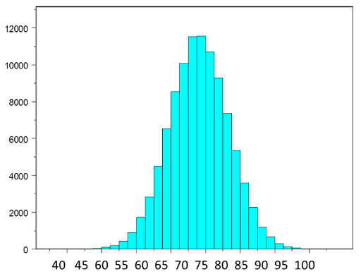
The figure below illustrates a normally distributed feature, X, in a population in which the population mean is 75 with a standard deviation of 8.
If nosotros accept simple random samples (with replacement) of size n=x from the population and compute the hateful for each of the samples, the distribution of sample means should exist approximately normal according to the Fundamental Limit Theorem. Note that the sample size (due north=10) is less than 30, merely the source population is usually distributed, so this is not a problem. The distribution of the sample means is illustrated beneath. Note that the horizontal axis is different from the previous analogy, and that the range is narrower.
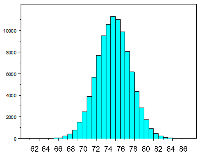
The hateful of the sample means is 75 and the standard deviation of the sample means is 2.v, with the standard departure of the sample means computed every bit follows:
If we were to take samples of n=5 instead of northward=10, we would get a like distribution, merely the variation among the sample means would exist larger. In fact, when nosotros did this nosotros got a sample mean = 75 and a sample standard departure = iii.vi.
Key Limit Theorem with a Dichotomous Upshot
Now suppose we measure a characteristic, X, in a population and that this feature is dichotomous (eastward.k., success of a medical procedure: yes or no) with 30% of the population classified as a success (i.due east., p=0.xxx) as shown beneath.
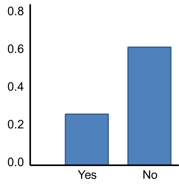
The Key Limit Theorem applies fifty-fifty to binomial populations like this provided that the minimum of np and n(1-p) is at least 5, where "north" refers to the sample size, and "p" is the probability of "success" on any given trial. In this case, we will take samples of n=twenty with replacement, so min(np, northward(ane-p)) = min(20(0.3), 20(0.7)) = min(6, 14) = 6. Therefore, the benchmark is met.
We saw previously that the population mean and standard difference for a binomial distribution are:
Mean binomial probability: 
Standard deviation: 
The distribution of sample ways based on samples of size n=20 is shown below.
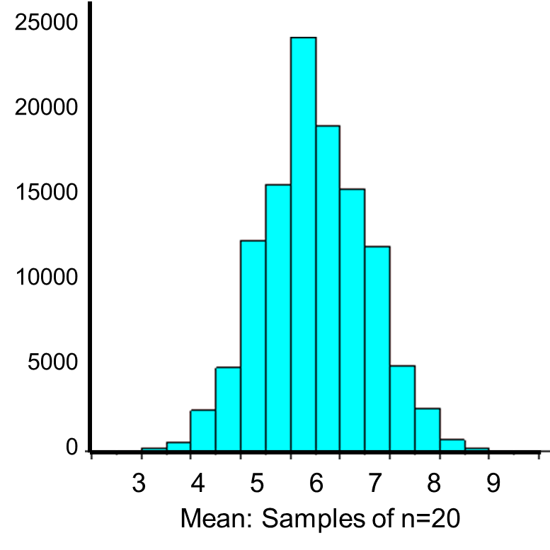
The mean of the sample means is
and the standard departure of the sample means is:
Now, instead of taking samples of due north=20, suppose we have simple random samples (with replacement) of size north=x. Note that in this scenario we do not meet the sample size requirement for the Central Limit Theorem (i.e., min(np, n(one-p)) = min(10(0.3), 10(0.7)) = min(3, seven) = three).The distribution of sample means based on samples of size n=10 is shown on the right, and you can see that it is not quite normally distributed. The sample size must be larger in order for the distribution to approach normality.
Central Limit Theorem with a Skewed Distribution
The Poisson distribution is another probability model that is useful for modeling discrete variables such every bit the number of events occurring during a given time interval. For instance, suppose you lot typically receive about iv spam emails per day, just the number varies from twenty-four hour period to day. Today you happened to receive 5 spam emails. What is the probability of that happening, given that the typical charge per unit is 4 per 24-hour interval? The Poisson probability is:
Mean = μ
Standard divergence = 
The mean for the distribution is μ (the average or typical charge per unit), "10" is the bodily number of events that occur ("successes"), and "eastward" is the constant approximately equal to 2.71828. So, in the example above
Now let's consider another Poisson distribution. with μ=3 and σ=one.73. The distribution is shown in the figure below.
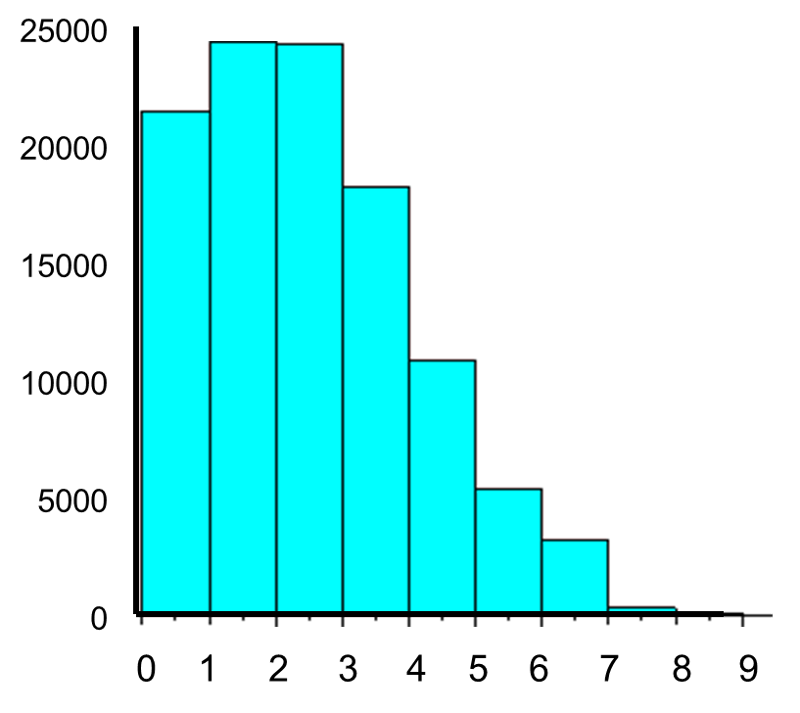
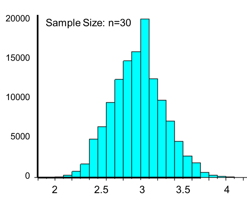
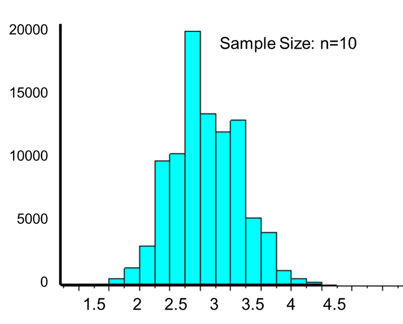
This population is not normally distributed, but the Central Limit Theorem will apply if northward > thirty. In fact, if nosotros accept samples of size due north=30, nosotros obtain samples distributed as shown in the kickoff graph below with a hateful of 3 and standard divergence = 0.32. In contrast, with minor samples of n=10, we obtain samples distributed as shown in the lower graph. Annotation that n=ten does not meet the benchmark for the Cardinal Limit Theorem, and the small samples on the right give a distribution that is not quite normal. As well notation that the sample standard deviation (too called the "standard error") is larger with smaller samples, considering information technology is obtained past dividing the population standard deviation by the square root of the sample size. Another mode of thinking most this is that extreme values will take less bear upon on the sample mean when the sample size is big.
Source: https://sphweb.bumc.bu.edu/otlt/mph-modules/bs/bs704_probability/BS704_Probability12.html
0 Response to "what does the central limit theorem have to do with normal distributions?"
Enregistrer un commentaire